Content

About

Data sources

• 1) Baseline data

• 2) Historical data

• 3) Future climate data

• 4) Paleoclimate data

• 5) How to add climate data from additional GCMs

Climate variables predicted

• 1) Annual variables

• 2) Seasonal variables

• 3) Monthly variables

How to download and install

How to use

• 1) Use the program interactively

• 2) For multi-location process

• 3) For Time Series

• 4) Read and output raster map files

• 5) Process the raster output files

• 6) Command-line operations

• 7) Call command line operations in R

• 8) Tutorial videos

About the package

ClimateBC is a standalone MS Windows software application (Wang et al. 2016) that extracts and downscales gridded (4 x 4 km) monthly climate data for the reference normal period (1961-1990) from PRISM (Daly et al. 2008) to scale-free point locations. It also calculates many (>200) monthly, seasonal and annual climate variables. The downscaling is achieved through a combination of bilinear interpolation and dynamic local elevational adjustment. ClimateBC also uses the scale-free data as a baseline to downscale historical and future climate variables for individual years and periods between 1901 and 2100. A time-series function is available to generate climate variables for multiple locations and multiple years.

The program can read and output comma-delimitated spreadsheet (CSV) files. It (since v6.00) can also directly read digital elevation model (DEM) raster (ASC) files and output climate variables in raster format for mapping. The spatial resolution of the raster files is up to user’s preference. The program (since v7.20) supports command line operations and can be called by other programs, such R or Python. The coverage of the program is shown in Figure 1.

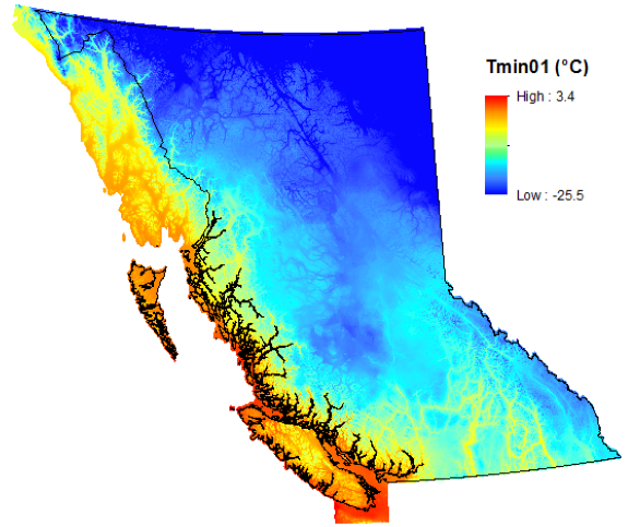
Figure 1. The coverage of ClimateBC.

Data sources

1) Baseline data

• PRISM at 800 x 800 m from Pacific Climate Impact Consortium;

• The monthly solar radiation data (1948-2010) were provided by Dr. Robbie Hember at University of British Columbia.

2) Historical climate data

Historical monthly data were developed by ourselves and replaced the data from Climate Research Unit (CRU ts4.01), which were used in previous versions, for improved accuracies. The data are at the spatial resolution is 0.5 x 0.5°.

3) Future climate data

The future climate projections were selected from the General Circulation Models (GCMs) of the Coupled Model Intercomparison Project (CMIP6) to be included in IPCC sixth assessment report (AR6). The new set of emissions scenarios from CMIP6, called “Shared Socioeconomic Pathways” (SSPs), included SSP126, SSP245, SSP460, SSP370 and SSP585. As of December 2020, there were 44 global climate models contributing to the CMIP6 ScenarioMIP project. We selected a subset of 13 of these models for ClimateBC/NA based on the following criteria: 1. Minimum of 3 historical runs available; 2. Tmin and Tmax available for all runs; 3. At least one run for each of the four main SSP marker scenarios; 4. One model per institution; 5. No closely related models, based on Fig. 5 in [Brunner et al. 2020] (https://esd.copernicus.org/articles/11/995/2020/esd-11-995-2020.html); and 6. No large biases over BC (resulted in only one exclusion: AWI-CM-1-1-MR). A tool to visualize and compare the projections of this ensemble is available for British Columbia at https://bcgov-env.shinyapps.io/cmip6-BC/.

We included three normal periods (2011-2040, 2041-2070, and 2071-2100) and five 20-year periods (2001-2020, 2021-2040, 2041-2060, 2061-2080, and 2081-2100). When multiple runs are available for each GCM, an average was taken over the available (up to 10) runs. Ensembles among the 13 GCMs are also available. Time-series of monthly projections for individual years are available for the period 2011-2100 with all the 13-GCM ensembles and 10 individual GCMs.

To address the “too hot” issues of some GCM projections, 8-GCM ensembles have been added for 30-year (normal) and 20-year averages, and annual periods. These new ensembles are generated from 8 GCMs that are within the IPCC's latest assessment of the “very likely” range of Earth's equilibrium climate sensitivity (ECS). The 8 GCMs include: ACCESS-ESM1-5, CNRM-ESM2-1, EC-Earth3, GFDL-ESM4, GISS-E2-1-G, MIROC6, MPI-ESM1-2-HR, and MRI-ESM2-0. Please click here for details.  

4) Paleoclimate climate data

Monthly paleoclimate data were from four GCMs of the CMIP5. The paleo periods covered: 1) Last Millennium or past 1000 years, starting on January 01, 0850; 2) MidHolocene (6,000 years ago); and 3) Last Glacial Maximum (21,000 kyrs ago). Monthly averages were taken over the first 50 years of each period, which is the minimum period available in among the four GCMs.

How to add climate data from additional GCMs

The coordinate file “ClimateBC_GCM_coord_vID.csv” included in the “Reference” folder can be used as a template to add additional GCM data to the package by users. After the monthly climate data are added to the template, remove the first three columns and save it to the GCMdat folder with the extension name “.gcm”. This applies to GCM time series data as well.

Climate variables predicted

1) Annual variables

Directly calculated annual variables:
	MAT	mean annual temperature (°C)
	MWMT	mean warmest month temperature (°C)
	MCMT	mean coldest month temperature (°C)
	TD	temperature difference between MWMT and MCMT, or continentality (°C)
	MAP	mean annual precipitation (mm)
	AHM	annual heat-moisture index (MAT+10)/(MAP/1000))
	SHM	summer heat-moisture index ((MWMT)/(MSP/1000))
Derived annual variables:
	DD<0 (or DD_0)	degree-days below 0°C, chilling degree-days
	DD>5 (or DD5)	degree-days above 5°C, growing degree-days
	DD<18 (or DD_18)	degree-days below 18°C, heating degree-days
	DD>18 (or DD18)	degree-days above 18°C, cooling degree-days
	NFFD	the number of frost-free days
	FFP	frost-free period
	bFFP	the day of the year on which FFP begins
	eFFP	the day of the year on which FFP ends
	PAS	precipitation as snow (mm). For individual years, it covers the period between August in the previous year and July in the current year
	EMT	extreme minimum temperature over 30 years (°C)
	EXT	extreme maximum temperature over 30 years (°C)
	Eref	Hargreaves reference evaporation (mm)
	CMD	Hargreaves climatic moisture deficit (mm)
	MAR	mean annual solar radiation (MJ m‐2 d‐1)
	RH	mean annual relative humidity (%)
	CMI	Hogg’s climate moisture index (mm)
	DD1040	degree-days above 10°C and below 40°C

2) Seasonal variables

Directly calculated annual variables:
	Tave_wt	winter mean temperature (°C)
	Tave_sp	spring mean temperature (°C)
	Tave_sm	summer mean temperature (°C)
	Tave_at	autumn mean temperature (°C)
	Tmax_wt	winter mean maximum temperature (°C)
	Tmax_sp	spring mean maximum temperature (°C)
	Tmax_sm	summer mean maximum temperature (°C)
	Tmax_at	autumn mean maximum temperature (°C)
	Tmin_wt	winter mean minimum temperature (°C)
	Tmin_sp	spring mean minimum temperature (°C)
	Tmin_sm	summer mean minimum temperature (°C)
	Tmin_at	autumn mean minimum temperature (°C)
	PPT_wt	winter precipitation (mm)
	PPT_sp	spring precipitation (mm)
	PPT_sm	summer precipitation (mm)
	PPT_at	autumn precipitation (mm)
	RAD_wt	winter solar radiation (MJ m-2 d-1)
	RAD_sp	spring solar radiation (MJ m-2 d-1)
	RAD_sm	summer solar radiation (MJ m-2 d-1)
	RAD_at	autumn solar radiation (MJ m-2 d-1)
Derived annual variables:
	DD_0_wt ~ DD_0_at	winter ~ Autumn degree-days below 0°C
	DD5_wt ~ DD5_at	winter ~ Autumn degree-days above 5°C
	DD_18_wt ~ DD_18_at	winter ~ Autumn degree-days below 18°C
	DD18_wt ~ DD18_at	winter ~ Autumn degree-days above 18°C
	NFFD_wt ~ NFFD_at	winter ~ Autumn number of frost-free days
	PAS_wt ~ PAS_at	winter ~ Autumn precipitation as snow (mm)
	Eref_wt ~ Eref_at	winter ~ Autumn Hargreaves reference evaporation (mm)
	CMD_wt ~ CMD_at	winter ~ Autumn Hargreaves climatic moisture deficit (mm)
	RH_wt ~ RH_at	winter ~ Autumn relative humidity (%)
	CMI_wt ~ CMI_at	winter ~ Autumn Hogg’s climate moisture index (mm)

Note: Winter (_wt): December, January and Februrary.  Spring (_sp): March, April and May.   Summer (_sm): June, July and August.  Autumn (_at): September, October and November. The December is from the previous year if the climate data is for a specific year instead of a multi-year period. 

2) Monthly variables

Primary monthly variables:
	Tave01 – Tave12	January - December mean temperatures (°C)
	Tmax01 – Tmax12	January - December maximum mean temperatures (°C)
	Tmin01 – Tmin12	January - December minimum mean temperatures (°C)
	PPT01 – PPT12	January - December precipitation (mm)
	Rad01 – Rad12	January - December solar radiation (MJ m-2 d-1)
Derived monthly variables:
	DD_0_01 – DD_0_12	January - December degree-days below 0°C
	DD5_01 – DD5_12	January - December degree-days above 5°C
	DD_18_01 – DD_18_12	January - December degree-days below 18°C
	DD18_01 – DD18_12	January - December degree-days above 18°C
	NFFD01 – NFFD12	January - December number of frost-free days
	PAS01 – PAS12	January – December precipitation as snow (mm)
	Eref01 – Eref12	January – December Hargreaves reference evaporation (mm)
	CMD01 – CMD12	January – December Hargreaves climatic moisture deficit (mm)
	RH01 – RH12	January – December relative humidity (%)
	CMI01 – CMI12	January – December Hogg’s climate moisture index (mm)

How to download and install

To download the package for free, please click here to register and obtain a download link. The size of the package is about 365 MB. No installation is required. Simply unzip all the files and subfolders into a folder on your hard disk and double-click the file ClimateBC _v6.**.exe”. The program does not run properly on network drives.

The program runs on all Windows. It can also run on Linux, Unix and Mac systems with the free software Wine or MacPorts/Wine.

How to use

1) Use the program interactively for single locations

Latitude and longitude can be entered in either decimal degrees (e.g. Lat: 51.542, Long: 129.333) or degree, minute and second (e.g., 51°30’15”N, 129°15’30’W). Longitude information is accepted either in positive or negative values. Elevation has to be entered in meters, or empty if no elevation data are available. If "Monthly variables", "Seasonal variables" or "All variables" output variables was selected, an additional output sheet appears and annual climate variables are still calculated.

Output data can be saved as a text file and imported to spreadsheet file using space-delimitated option. 

2) Use the program interactively for single locations

Most users will have their sample data information in an Excel spreadsheet or in a text file. To make it possible for the program to read this data it must first be modified to a standard format. 

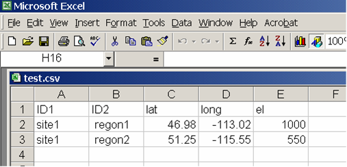
Create a spreadsheet with the headers “ID1, ID2, lat, long, el” as shown in the example below. ID1 and ID2 can be “Location”, “Region” or whatever. The file must have the title row and all variables in the same order as shown. If you don’t have elevation information or a second ID, you have to put in “.” in the columns. If you have more information columns in your original file, you have to remove them.  

If you use a GPS or GIS software to obtain your location information for many samples latitude values in the western hemisphere will be negative. For convenience, you can use either positive or negative values, and the program will automatically convert the data. 

After the spreadsheet is prepared as shown, save it as “comma delimited text file” by choosing “Save as …” from the file menu, and then specifying (*.csv) from the “Save as type …” drop-down menu. 

You can also directly create a comma delimited text file in any text editor such as Notepad. If there is a missing value, you need to enter a “.” between two commas.  

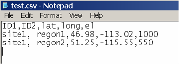
 Save this text file with a .csv extension by writing out the full file name with extension in parenthesis when saving, e. g. “test.csv” instead of test.csv or test. 

 Now you are ready for processing: Click on "Select input file" button to read your spreadsheet and on "Specifiy output file" button to specify your output file folder and file. Then, click the "Start" button. Climate variable information will be appended as additional columns to your input file. If elevation information is provided the climate variables will be elevation adjusted.

3) For Time Series

Time Series function works only for the multi-location process. To process a single location, you need to have the location in your input file. Here are the steps to follow:  

1. Select “Time Series” (for historical years) or a future time series in the period section drop box;
2. Select a variable category (monthly, seasonal, annual or all variables);
3. Input the starting and ending years in the pop-up boxes;
4. Specify input and output files, and click the “Calculate TS” button.

4) Read and output raster map files

1. Have a DEM raster file (*.asc) for the area of interest at the resolution you want. The raster file is required to be in a latitude-longitude projection (WGS84), prepared in ArcGIS or in R (QGIS format is not supported), and please make sure that the ASC file has proper line breaks (Windows format only). Here is the R code to convert a raster in TIF to ASC:

Library(raster)

tif <- raster('C:/data/dem.tif')

NAvalue(tif) <- -9999

writeRaster(tif, 'C:/data/dem.asc',overwrite=TRUE)  

 

If you use terra package, you need an extra step:

library(terra)

tif <- rast('C:/data/dem.tif')

writeRaster(r, 'dem0.asc',NAflag=-9999,overwrite=TRUE)

temp <- readLines('dem0.asc')

write.table(temp,'dem.asc', row.names=F,col.names=F,quote=F)

 

2. Click the “Select input file” button and a file open box will show up.
3. Navigate to the folder containing the raster file;
4. Select the File type: “asc” as shown in the following screenshot and only asc raster files will show up: 



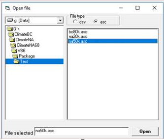
5. Select an asc input file and click “Open” button.
6. Click the “Specify output file” button, and a default folder will show up.
7. Click the “Save” button.
8. Click the “Start” button, and climate variables in ASCII raster format will be generated.

5) Process the raster output files

The output asc raster files can be directly imported (drag/drop) to ArcGIS or other GIS programs to generate maps. They can also be directly used in R to plot maps using the following code as an example:  

6) Command Line operations

In CMD prompt, navigate to the directory of the program, and type: 

         ClimateBC_v7.41.exe /Y /Normal_1961_1990.nrm /1_test.csv /test_normal.csv

Where 

7) Call command line operations in R

Here is an R code example to call the program in R: 

8) Tutorial videos

https://www.youtube.com/channel/UC6v_vfKWSZ_o05Ud-yscj7Q/video 

---